CSG for engineering

Engineering models are not two clean solids. A ground model is a block, a terrain, faults, horizons that stop at them, ore bodies and a tunnel in 420 slices. A CFD setup is a tunnel box, refinement zones and a vehicle shell that crosses itself. The meshes are open. They overlap. They touch along whole planes.

trueform's CSG graph takes all of them at once. One exact build cuts every operand against every other. After that, any region is one read: a rock unit, the rock the drive takes, the fluid around a body. Each comes back as a closed mesh, every face traced to its source. The domains are conformal: neighbouring regions share their interface triangle for triangle.

CAD meshers call this a fragment or a general fuse. trueform does it on triangle meshes, as they come from scans, exports and modellers. For two meshes and one answer, see mesh booleans. Dig a tunnel through layered ground in the live example.

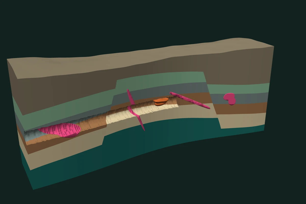
Synthetic data 445 operands · 19 sheets · one graph

What comes back

An engineer rarely wants one mesh. One graph returns all of these:

• Conformal domains. Every region the surfaces enclose, each a closed mesh with a stable id, meeting its neighbours on the same triangles. Each can take a material, a boundary condition or a volume.
• An inclusion matrix. One row per domain, one column per operand: inside or outside.
• Regions. Domains picked by a boolean expression, or by a mask over the matrix.
• Surfaces. One operand's walls of a region, or the part of a surface that lies inside one.
• Provenance. For every output face, the operand and the input face it came from.

A model for simulation needs conformal domains. Two regions that touch must share one interface: the same points, the same triangles, no gap and no overlap between them. Interfaces that almost agree leave slivers and holes that a solver cannot use.

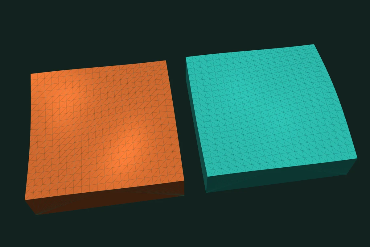
The graph returns them that way. Below, a block is cut by a wavy horizon sheet into two domains, and the upper one is turned over like the page of a book. The two faces of the interface are mirror images, triangle for triangle, with identical coordinates. Weld the coincident points and the two domains share one interface, not two that almost agree.

Load the model as it is

The graph takes inputs as they come. Where only the engineer knows the intent, the engineer declares it.

Open surfaces cut. A horizon, a fault or a terrain has a rim and bounds no volume. List it in sheets and it becomes an oriented separator. It cuts and is cut like any other operand, and op(i) means the side behind its normal. A volume cut by a sheet comes back closed, capped by the sheet.

Shells that overlap themselves. One file can hold several shells that cross each other: instanced parts that touch, a merged export. Pass within=True and the graph also cuts each operand against itself.

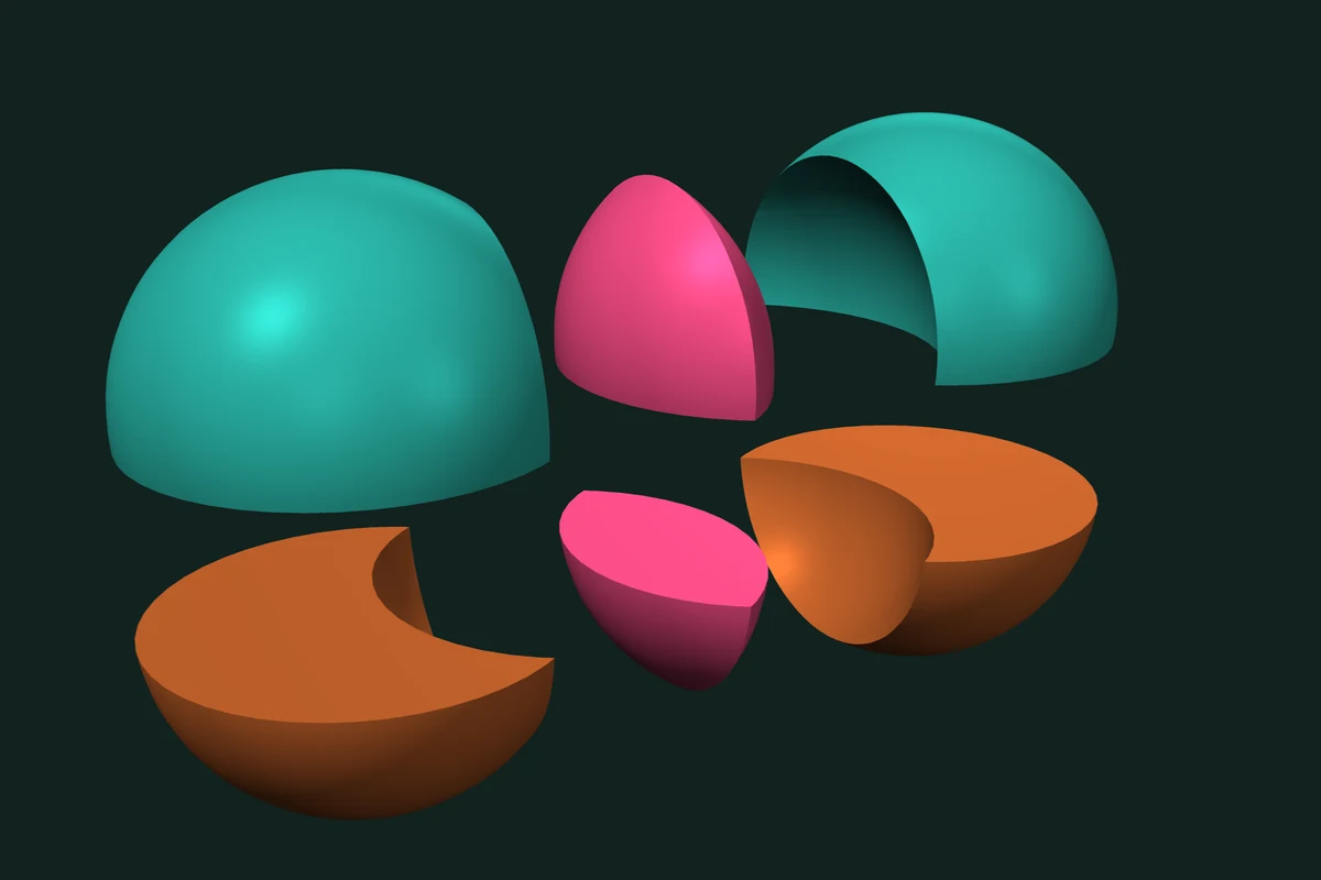
In the picture, operand 0 is two overlapping spheres stored as one mesh and operand 1 is a slab. domains() returns six cells: each sphere's own part and the lens, above the slab and inside it. Expressions still read each operand as one solid; to name a self-overlapping operand in one, repair it first with outer_shell.

Faces that coincide. Where two layers touch, their faces lie in one plane. The graph classifies coincident faces exactly, as it does for two meshes. The tests on mesh booleans show what that means.

Surfaces that fall short. A horizon that stops before it reaches a fault seals nothing. The graph does not guess a side for it. sheet_rim_volumes lists every sheet whose free rim ends inside a volume, with that volume, so an empty region is never silent.

Faces that disagree on their winding. Each volume operand needs a clear inside, so neighbouring faces must agree. Orient them before the build with orient_faces_consistently.

Build once, read many times

The build computes one exact arrangement of all operands and classifies every region against every operand. Every read reuses it. A chain of pairwise booleans instead starts over from each new mesh.

On the public N-ary benchmark, a union of 64 Thingi10K meshes, trueform builds the arrangement in 103 ms median: 14× faster than Solidean and Manifold, 44× Cherchi, 138× MeshLib, 536× CGAL and 648× Geogram. Apple M4 Max, 16 threads, trueform 0.9.8.

C++up to 648× faster

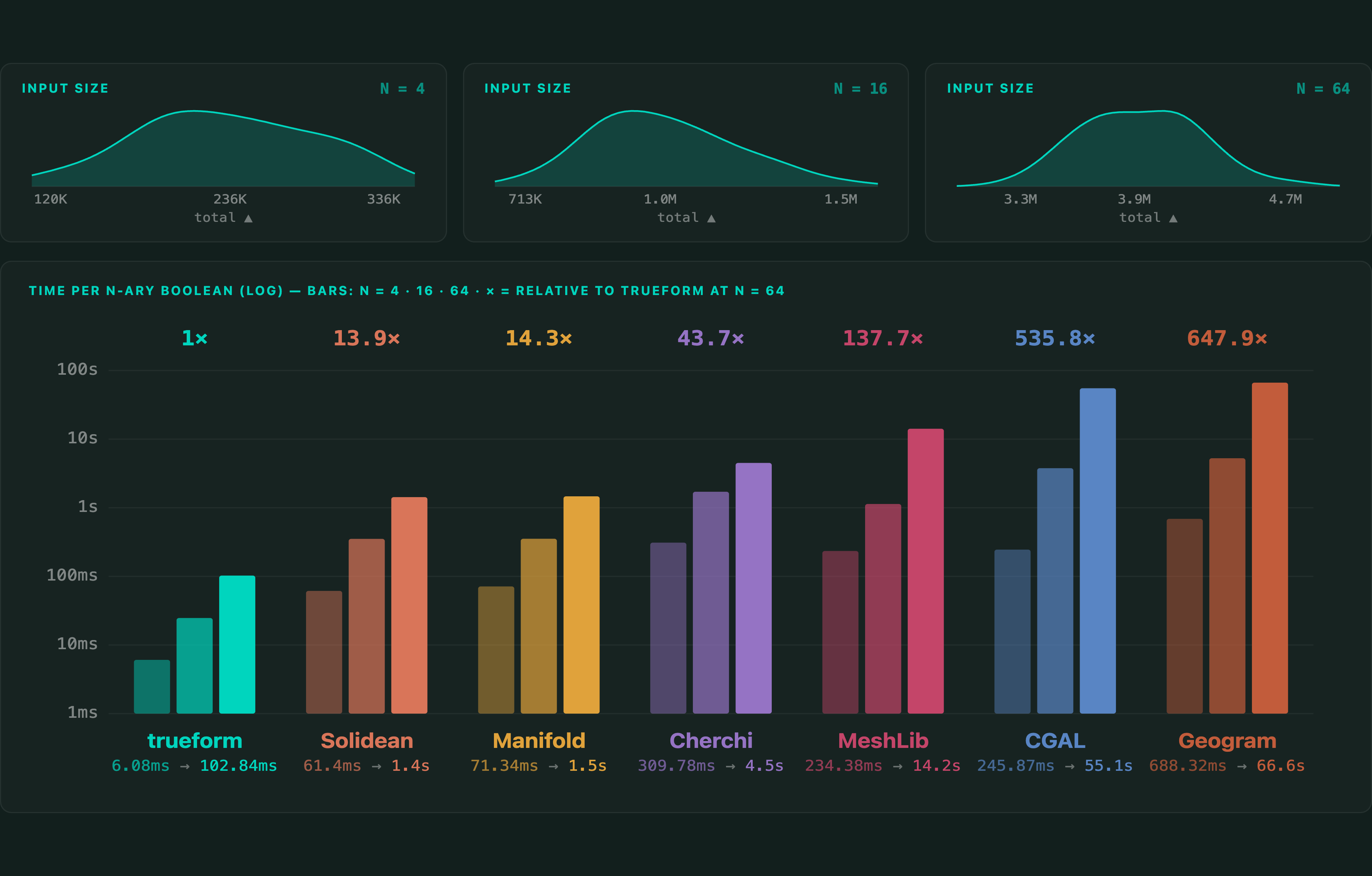
Full tables and protocol: Mesh Boolean Library Comparison and Benchmarks — 2026. One graph over 201 meshes, many expressions: the variadic tutorial. Every module: the trueform benchmarks page.

A tunnel drive, slice by slice

The ground model at the top of this page is synthetic, in local metres, with 445 operands in one graph:

• the ground volume and the terrain;
• two faults, with the rock offset across them;
• 15 horizon pieces, five per fault block, bounding six rock units;
• a cavity and four ore bodies;
• 420 excavation slices, 0.5 m each, along a curved alignment;
• a curtain sheet that cuts the model away along its length for display.

Nineteen of the operands are sheets: the terrain, the faults, the horizons and the curtain.

A rock unit is an expression. In each fault block it lies below its top horizon and above the one beneath. The cavity and every ore are subtracted, so each volume of rock is counted once. The excavation after n slices is the union of the first n slices. The rock a unit loses to the drive is one more intersection.

# GROUND, TERRAIN, F0, F1, CAVITY, ORES, FIRST_SLICE and horizon(b, k)
# are operand indices in `meshes`.
graph = tf.CsgGraph(meshes, sheets=sheets)       # 445 operands, built once

def unit(k):
    # rock unit k: between its horizons in each fault block,
    # inside the ground, minus the cavity and every ore
    blocks = [tf.op(F0), ~tf.op(F0) & tf.op(F1), ~tf.op(F1)]
    e = None
    for b in range(3):
        top = tf.op(horizon(b, k)) if k < 5 else tf.op(TERRAIN)
        part = blocks[b] & top
        if k > 0:
            part = part - tf.op(horizon(b, k - 1))
        e = part if e is None else e | part
    e = tf.op(GROUND) & e - tf.op(CAVITY)
    for ore in ORES:
        e = e - tf.op(ore)
    return e

def dug(n):
    # the first n excavation slices
    e = tf.op(FIRST_SLICE)
    for i in range(FIRST_SLICE + 1, FIRST_SLICE + n):
        e = e | tf.op(i)
    return e

for n in range(1, 421):                          # as the face advances
    for k in range(6):
        faces, points = graph.mesh(unit(k) & dug(n))
        excavated = tf.volume(tf.Mesh(faces, points))

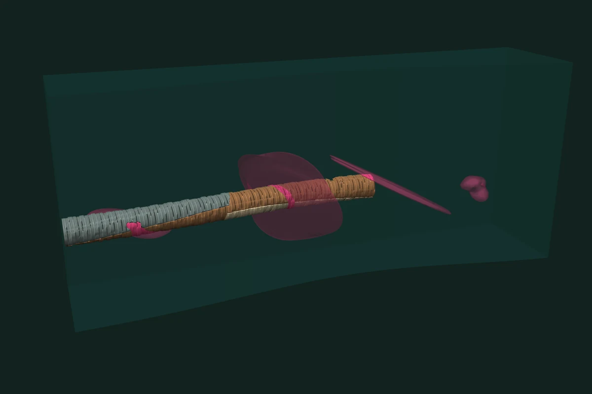
One build serves all 420 reads, fast enough to follow the drive as it advances. The six units plus the four ores add up to the ground below the terrain minus the cavity: nothing is counted twice and nothing is lost.

Fluid domains and finite element models

The pattern is not specific to ground. A wind-tunnel box, a refinement zone and a vehicle make a CFD setup. The fluid domain is the box minus the vehicle. The near-field and wake region is the zone minus the vehicle. Both come from one graph as conformal domains: they meet on shared triangles.

The car below is a public body shell as it was uploaded: closed, 282,570 triangles, with 246 pairs of faces that cross. outer_shell repairs it in one call, and it goes into the graph as is.

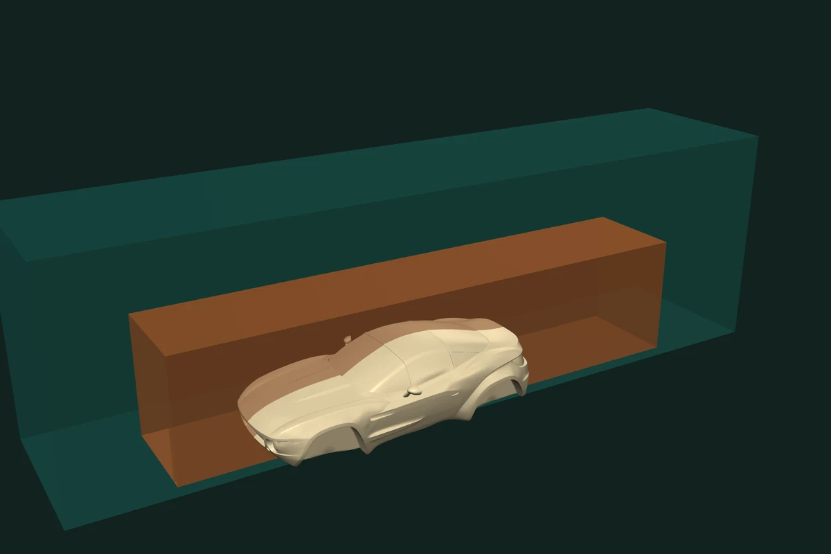
car = tf.outer_shell(car)                      # drops the self-crossings
graph = tf.CsgGraph([tunnel, zone, car])

far_field = graph.mesh(tf.op(0) - tf.op(1) - tf.op(2))
near_field = graph.mesh(tf.op(1) - tf.op(2))

Rally Fighter Body by LocalMotors, Thingiverse 40862, CC BY

For a finite element model, the conformal domains are the material regions, and each domain's row in the inclusion matrix says which parts contain it.

Read surfaces, not only volumes

Sometimes the answer is an area. The part of a horizon inside an excavation is a contact surface. The walls of one unit carry a load. Two keywords read them off the same build:

• selection=[i] returns the faces of operand i that bound the region, wound outward.
• inside=[i] returns the surface of operand i that lies inside the region, in its own winding.

# operand BOX is a unit box, operand PLANE a sheet through its middle
faces, points = graph.mesh(tf.op(BOX), inside=[PLANE])                  # the cap: area 1.0
faces, points = graph.mesh(tf.op(BOX) - tf.op(PLANE), selection=[BOX])  # walls above: area 3.0

Pass return_source_ids=True to any read and every output face also carries its operand and its input face. Colours, materials and survey attributes then follow the cut.

The graph in code

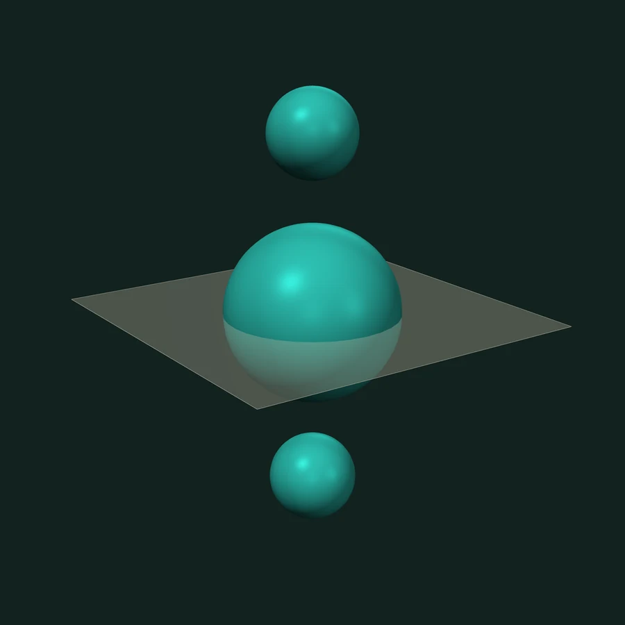
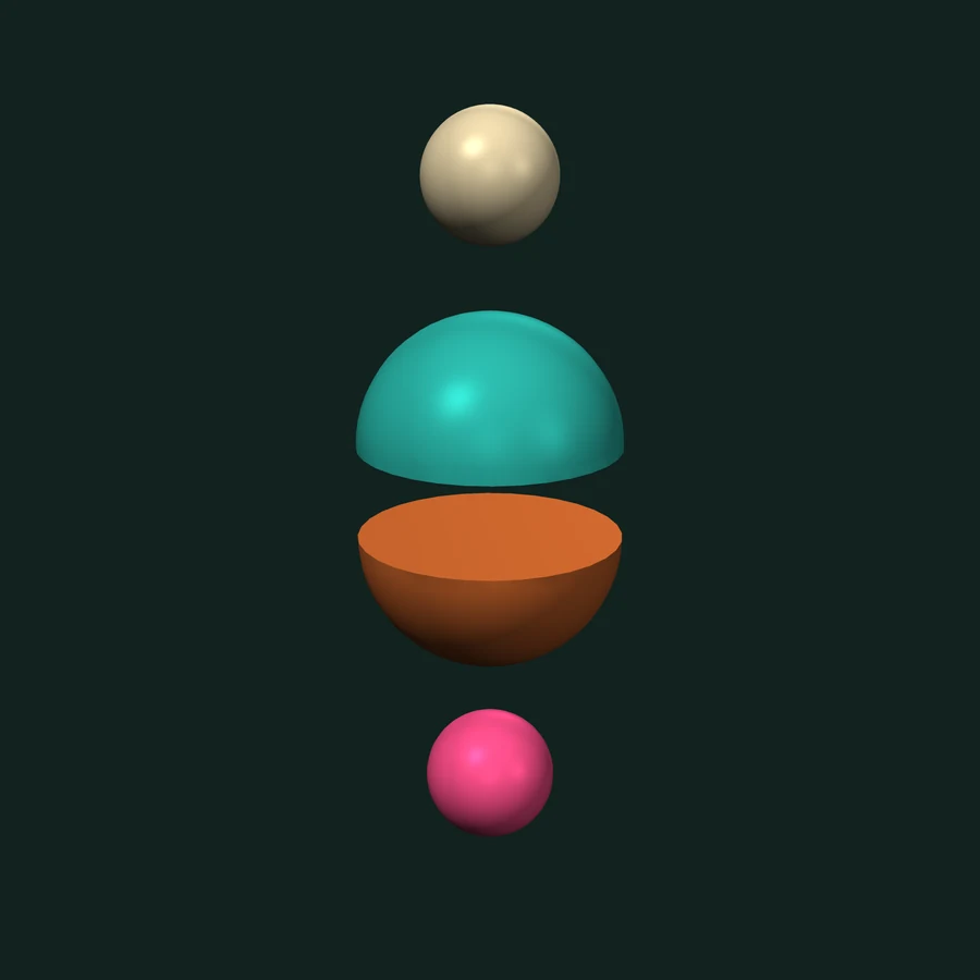
The trueform docs teach the graph with one small scene: Booleans and Domains from One Build. A sphere straddles a flat knife. Two smaller spheres float above and below it and touch nothing. The knife is declared a sheet, so op(3) means below it. One build answers three questions.

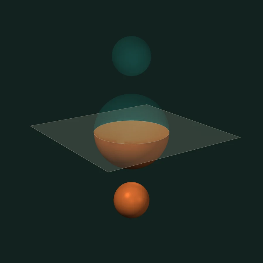
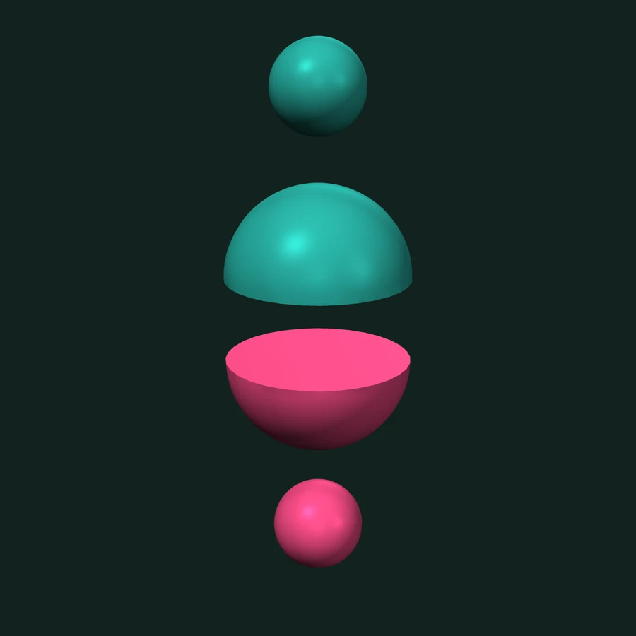
import numpy as np
import trueform as tf

def sphere(center, radius):
    sf, sp = tf.make_sphere_mesh(radius, 32, 32)
    return tf.Mesh(sf, np.asarray(sp) + np.asarray(center, sp.dtype))

plane_faces, plane_points = tf.make_plane_mesh(4.0, 4.0)
meshes = [sphere((0, 0, 0), 1.0),      # op 0: straddles the knife
          sphere((0, 0, 2), 0.5),      # op 1: floats above
          sphere((0, 0, -2), 0.5),     # op 2: floats below
          tf.Mesh(plane_faces, plane_points)]  # op 3: the knife

graph = tf.CsgGraph(meshes, sheets=[3])
solids = tf.op(0) | tf.op(1) | tf.op(2)

# 1. boolean meshes: one closed mesh per side
above_mesh = graph.mesh(solids - tf.op(3))
below_mesh = graph.mesh(solids & tf.op(3))

# 2. domains by expression: the same volumes, one mesh each
above_cells, above_ids = graph.domains(solids - tf.op(3))
below_cells, below_ids = graph.domains(solids & tf.op(3))

# 3. domains by hand: extract once, select by mask
cells, ids, imap = graph.domains(return_index_map=True)
below = imap.inclusion[:, 3]
above = ~below

#include <trueform/trueform.hpp>

auto straddle = tf::make_sphere_mesh<int>(1.f, 32, 32);
auto above_s  = tf::make_sphere_mesh<int>(0.5f, 32, 32);
auto below_s  = tf::make_sphere_mesh<int>(0.5f, 32, 32);
auto plane    = tf::make_plane_mesh<int>(4.f, 4.f);

auto at = [](float z) {
  return tf::make_frame(tf::make_transformation_from_translation(
      tf::vector<float, 3>{0.f, 0.f, z}));
};
std::vector forms{straddle.polygons() | tf::tag(at(0)),   // op 0
                  above_s.polygons()  | tf::tag(at(2)),   // op 1
                  below_s.polygons()  | tf::tag(at(-2)),  // op 2
                  plane.polygons()    | tf::tag(at(0))};  // op 3: the knife

std::array<int, 1> sheets{3};
auto graph = tf::make_csg_graph(tf::make_range(forms), tf::make_range(sheets));
auto solids = tf::csg::merge(tf::csg::merge(0, 1), 2);

// 1. boolean meshes
auto above_mesh = tf::make_csg_mesh(graph, tf::csg::difference(solids, 3));
auto below_mesh = tf::make_csg_mesh(graph, tf::csg::intersection(solids, 3));

// 2. domains by expression
auto [above_cells, above_ids] =
    tf::make_csg_domains(graph, tf::csg::difference(solids, 3));

// 3. domains by hand: imap.inclusion[k][3] is true below the knife
auto [cells, ids, imap] = tf::make_csg_domains(graph, tf::return_index_map);

import * as tf from "@polydera/trueform";

function sphere(z: number, radius: number) {
  const m = tf.sphereMesh(radius, 32, 32);
  m.points.add_(tf.ndarray(new Float32Array([0, 0, z]), [3]));
  return m;
}
const meshes = [sphere(0, 1.0),       // op 0: straddles the knife
                sphere(2, 0.5),       // op 1: floats above
                sphere(-2, 0.5),      // op 2: floats below
                tf.planeMesh(4, 4)];  // op 3: the knife

const graph = tf.csgGraph(meshes, { sheets: [3] });
const solids = tf.op(0).or(1).or(2);

// 1. boolean meshes
const aboveMesh = graph.mesh(solids.sub(3));
const belowMesh = graph.mesh(solids.and(3));

// 2. domains by expression: { meshes, ids }
const above = graph.domains(solids.sub(3));
const below = graph.domains(solids.and(3));

// 3. domains by hand: a mask over the inclusion matrix
const all = graph.domains({ returnIndexMap: true });
const belowCells = all.meshes.filter((_, k) => all.inclusion.data[k * all.nTags + 3]);

One mesh per side. Each side comes back as one closed mesh: the straddler's half, capped by the knife, plus the floater on that side. Both sides have volume 2.5949. Use this when you want one surface, such as rock to export.

One mesh per domain. The same volumes, now as separate cells: two above, two below. Each cell is its own closed mesh. Use this when each region needs its own material, volume or mesh.

A mask over the matrix. Extract every domain once. Then any selection is a mask over the inclusion matrix. The knife's column says which cells lie below it. Ids are stable across reads of one graph, so the mask and the expression pick the same cells. Use this when a program, not a person, decides what to keep.

If you know fragments

Engineering tools have names for these steps. Here is how they map.

The difference is the input. A CAD kernel splits B-rep solids and surfaces. The graph splits triangle meshes, open or closed, as they come from scans, exports and implicit modellers. CAD solids go in tessellated.

Fields: buffers, blends and slices

Some work is easier on a grid. A buffer zone around an ore body is an offset surface. A scan may already be a field. The volume module samples a closed mesh into a signed distance field, combines fields by union, intersection and difference, extracts a level set by flying edges or dual contouring, and draws contour lines on any plane.

# ore_mesh, block_mesh: closed meshes, e.g. domains read off the graph
dims, spacing, origin = (96, 96, 48), (0.025,) * 3, (-1.2, -1.2, -0.6)

ore_field = tf.mesh_sdf(ore_mesh, dims, spacing, origin)
rock_field = tf.mesh_sdf(block_mesh, dims, spacing, origin)

buffer = tf.isosurface(ore_field, 0.1)          # 0.1 outside the ore
rock = tf.volume_boolean(rock_field, ore_field, "difference")
faces, points = tf.isosurface(rock, method="dual_contouring")  # keeps edges sharp

paths, points = tf.volume_slice_contours(       # a vertical section through the ore
    rock, plane_origin=(-1.2, 0.1, -0.6), u=(1, 0, 0), v=(0, 0, 1),
    dims2=(96, 48), spacing2=(0.025, 0.025), isovalues=0.0)

#include <trueform/trueform.hpp>
#include <trueform/volume.hpp>

auto field = [](const auto &polygons) {
  return tf::make_mesh_sdf(polygons, {96, 96, 48},
                           tf::point<float, 3>{0.025f, 0.025f, 0.025f},
                           tf::point<float, 3>{-1.2f, -1.2f, -0.6f});
};
auto ore_field = field(ore.polygons());
auto rock_field = field(block.polygons());

auto buffer = tf::make_isosurface(ore_field.volume(), 0.1f);
auto rock = tf::make_boolean(rock_field.volume(), ore_field.volume(),
                             tf::volume_boolean_op::difference);
auto surface = tf::make_isosurface(rock.volume(), 0.f,
                                   tf::isosurface_method::dual_contouring);

auto slice = tf::make_volume_slice(rock.volume(),
                                   tf::point<float, 3>{-1.2f, 0.1f, -0.6f},
                                   tf::point<float, 3>{1.f, 0.f, 0.f},
                                   tf::point<float, 3>{0.f, 0.f, 1.f},
                                   {96, 48}, {0.025f, 0.025f});
auto section = tf::make_isocontours(slice.volume(), 0.f);

A field boolean is bounded by the grid's spacing. The graph's boolean has no grid. Use fields for offsets, blends and resampling. Use the graph when the meshes must come back as they went in. See the volume docs.

Where to go next

• Two meshes. Mesh booleans: the hard-input tests, the speed of a single boolean, and code in three languages.
• Tutorial. Fast Variadic Mesh Booleans in C++: one graph over 201 meshes, many expressions. The pairwise tutorials in C++, Python and JavaScript use the same module.
• Docs. The CSG module, with sheets, selections, domains and the inclusion matrix, in C++, Python and TypeScript. The worked example: Booleans and Domains from One Build (C++ version).
• Method. Fast and Exact Mesh Booleans and Arrangements.

The CSG graph is one module of trueform. The same engine does spatial queries, topology, remeshing and more, in C++, Python and the browser.

@article{polydera:csg-for-engineering,
  title={CSG for engineering},
  author={Sajovic, {\v{Z}}iga, Polydera},
  year={2026},
  url={https://polydera.com/algorithms/csg-for-engineering},
  organization={Polydera}
}